
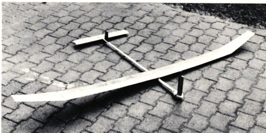
F1E Glider Model "Super Luckystar"
F. Tapernoux’s two second-place finishes at the 1976 regional and national slope competitions prove that large-scale magnetic models are the right choice. These models are suitable for calm weather with wind speeds of up to 6 m/sec.
The model’s speed can be adjusted by moving the wing and adding lead underneath it. You can record the speeds yourself in a table as follows:
Choose a day when the wind speed is as low and steady as possible—preferably early in the morning or in the evening. Next, select a slope that allows for flights of approximately 200 m. Now all you need is an anemometer. If you don’t have one, you can make do with a few strips of silver foil attached to a rod about 3 m long. These should always register the same deflection during a test flight. A well-tested model has a sink rate of approximately 0.3 m/sec. Once preparations are complete, you can proceed with the first flight. The model’s airspeed is approximately 3 m/sec. Using a 1:25,000 map, you should sketch a longitudinal profile of the selected area. Keep in mind that the slope should be as long and straight as possible and not hilly (to avoid the effects of gusts). You can now theoretically determine the landing point.
Starting height: 10 m
; Sink rate: 0.3 m/sec;
Wind speed: 0 m/sec;
Model speed: 3 m/sec.
$$a) \text{ Time} = \frac{1}{0.3} = 33.3 \text{ seconds}$$
$$b) \text{ Distance} = 33.3 \cdot 3 = 99.9 \text{ m} \sim 100 \text{ m}$$
During a flight, both the anemometer and the model should be observed simultaneously. After 3 trials, we enter the average value into a table and mark the point where the wing meets the fuselage. For the second series of tests, we move the wing back by 5 mm, increase the angle of attack by one turn using the elevator control screw at the rear (M2), and add an additional 50 grams of lead to the center of gravity.
In these flight tests, the landing point should be in the same location, i.e., at 100 m. Only the flight time is now shorter at the same wind speed, e.g., 25 seconds.
Mathematically, this follows:
$$V_s = \frac{\text{distance}}{\text{time}} = \frac{100}{25} = 4 \text{ m/sec}$$
i.e., at a wind speed of 3 m/sec, the model would fly forward at 1 m/sec.
We then move the wing back another 5 mm. Increase the angle difference. Add lead. We enter all the values obtained into a table.
This table is then a useful tool during competitions.
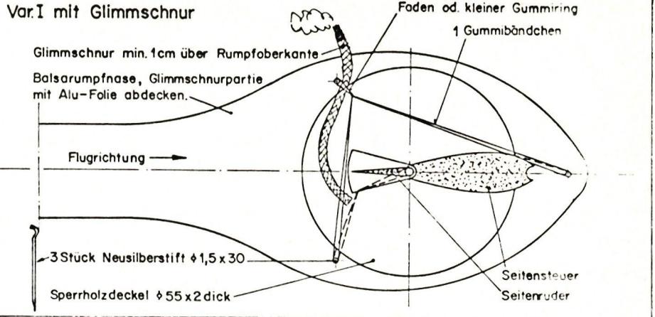
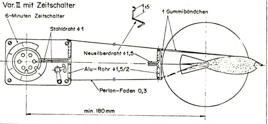
For the sake of completeness, I would like to discuss the circling method. The following two images show two variations:
- With a glow cord
- With a timer
Variation 1: The rudder of the Mamosteuering is locked in position after the desired time has elapsed using a taut rubber band. The lock can be released using the same wick by burning through the rubber.
Variation 2: With the timer switch, a second disc must be fabricated to release the rudder lock. Both discs must be adjustable relative to each other. Using the original disc and the wire mechanism, the rudder can be locked in place with the pre-tensioned rubber band. With the second disc, the rudder can be released again by ejecting the tensioned rubber band.
Here’s how this works in practice during flight:
- 2 minutes of straight flight = 1st function
- 2 minutes of circling (locked position) = 2nd function
- 1-minute straight flight = 3rd function
- = 5 minutes = Maximum flight with a landing not far from the launch site
Such an ideal flight certainly requires some practice, and only experienced magnet pilots will use this tactic.
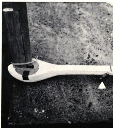
For magnetic model airplanes that tend to go into a spiral dive when circling, the shift in the center of gravity must also be taken into account. The simplest method: Clip a fishing sinker weighing about 15–20 g onto an S-shaped silver steel wire. A longer rubber band is attached to the side of the fuselage at approximately the height of the wing tips. Threaded through an eyelet, the rubber band is stretched to the control release point, where the sinker is attached. See photo. When the side control is locked, the fishing sinker snaps forward to the eyelet; its longitudinal position must be adjusted through trial and error.
Everyone can now see that achieving good performance in magnetic flight is not left to chance; rather, the model must be optimized in terms of topography, wind, and technology to achieve the best possible balance.
At this point, I will refrain from providing a detailed building description, as the model is constructed in virtually the same way as the Luckystar (see description in MFS, August 1973).
The magnet head is machined directly from a single piece of material along with the fuselage. The cover for the upper fuselage section, made from a 2-mm plywood sheet, also serves as a support for the sliding wing. Use lightweight wood! Remember, the wing does not need to withstand high launch forces. Weight of the finished model: 450 g. Payload: up to 300 grams of lead.
There is no 1:1 scale construction plan.
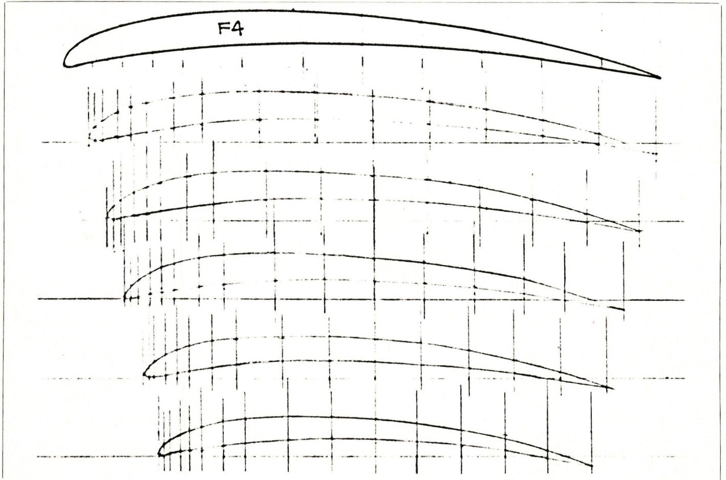
Nose radius 0.65
Graph paper is best suited for drawing the wing profile.
Example: For a wing depth of 16 cm, multiply the corresponding coordinate value by 1.6.
| x | = | 0 | 1.25 | 2.5 | 5 | 7.5 | 10 | 15 | 20 | 30 | 40 | 50 | 60 | 70 | 80 | 90 | 100 |
|---|---|---|---|---|---|---|---|---|---|---|---|---|---|---|---|---|---|
| yo | = | 0.68 | 2.80 | 3.84 | 5.34 | 6.43 | 7.20 | 8.38 | 9.06 | 9.65 | 9.45 | 8.78 | 7.78 | 6.31 | 4.21 | 1.45 | -2.0 |
| yu | = | 0.68 | 0.16 | 0.34 | 0.84 | 1.27 | 1.70 | 2.44 | 3.06 | 3.95 | 4.15 | 3.94 | 3.44 | 2.57 | 1.37 | -0.15 | -2.0 |

TEAM MANAGER "THIS" BOSSHARD
 Rodito Nussbaumer
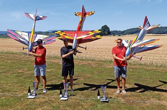
52. 2026 ALPS CUP
 Emil Giezendanner
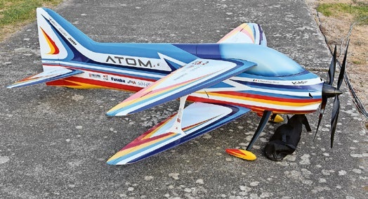
ATOM, THE NEW DOUBLE-DECKER FROM CPLR
 Matthias Bosshard
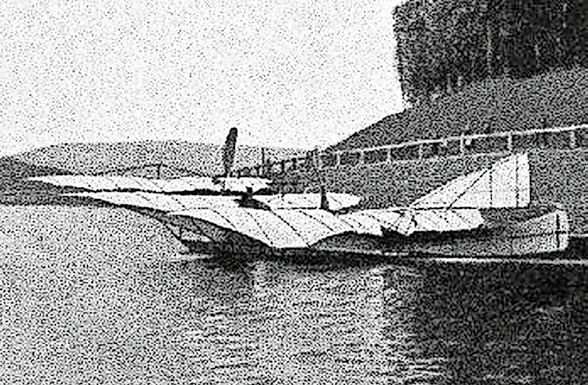
INSIGHTS INTO THE HISTORY OF SEAPLANES
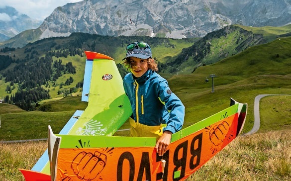
34th HAHNENMOOS ALPINE MODEL AIRPLANE CAMP
Res Dauwalder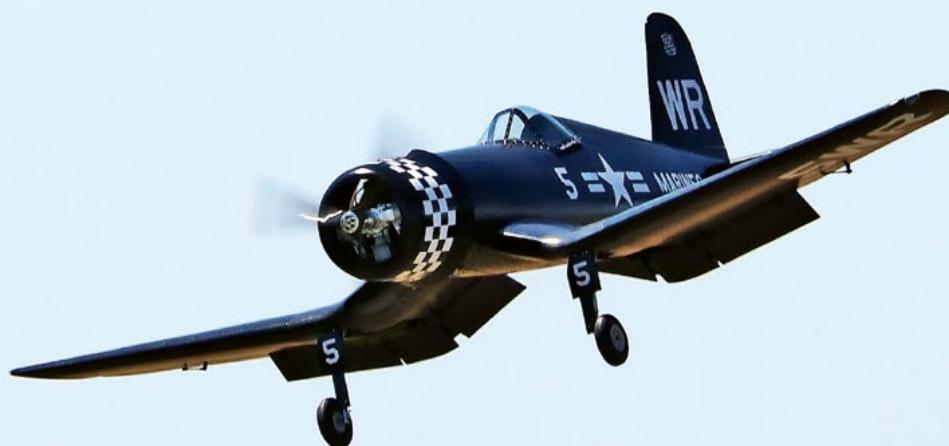
CORSAIR F4U – A WARBIRD WITH A MEMORABLE LOOK
Jürgen Rosenberger, Jürgen Prinz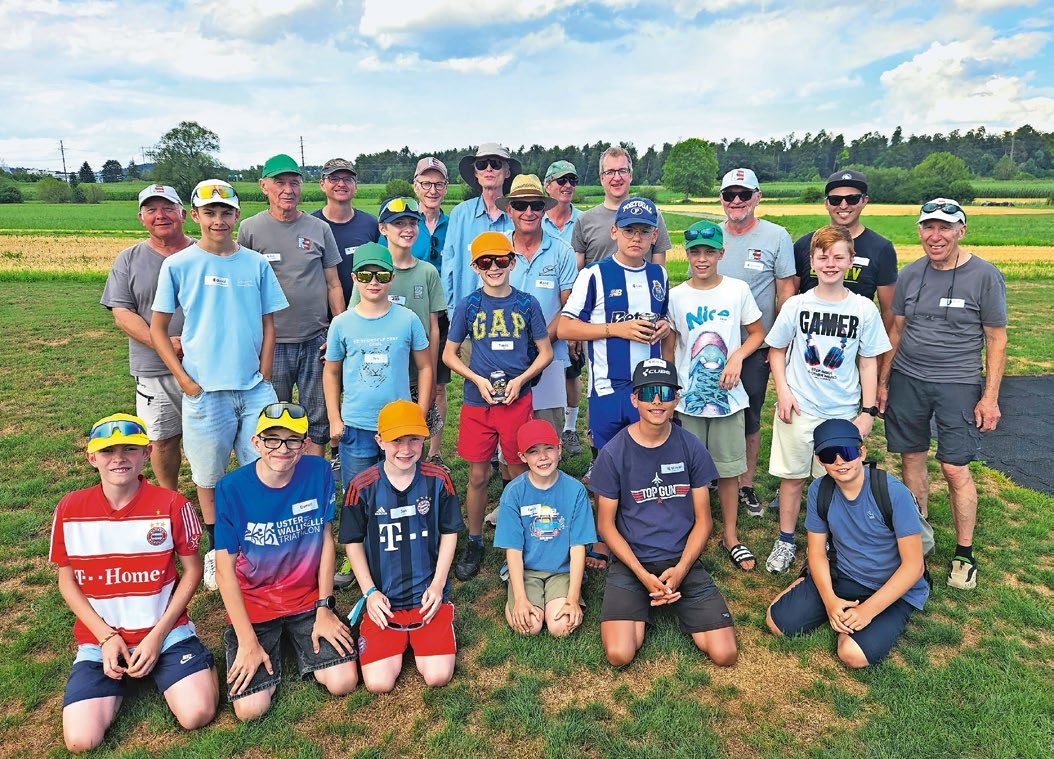
SUMMER FUN 2026 AT MG USTER
Martin Wunderli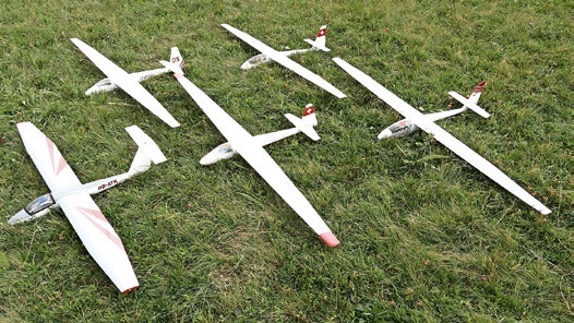
SMALL, MODEL-LIKE SAILBOATS
Res Dauwalder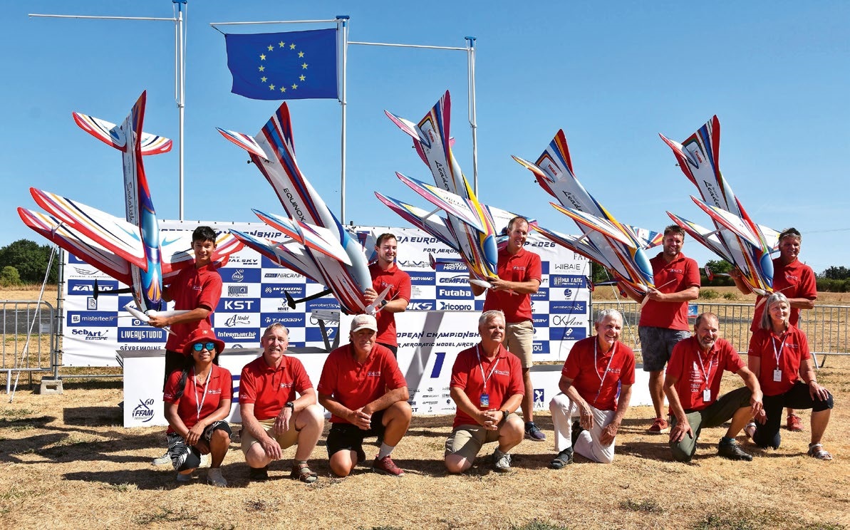
F3A EUROPEAN CHAMPIONSHIPS IN ST-MACAIRE, FRANCE
Matthias Bosshard
What's New at Leomotion.com
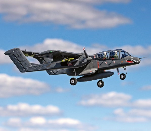
HORIZON HOBBY/LEMACO NEWS: MICRO OV-10 BRONCO 645 MM BY E-FLITE

PRIDE AND GOOD IDEAS
 Markus Nussbaumer
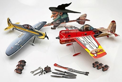
News from HEBU
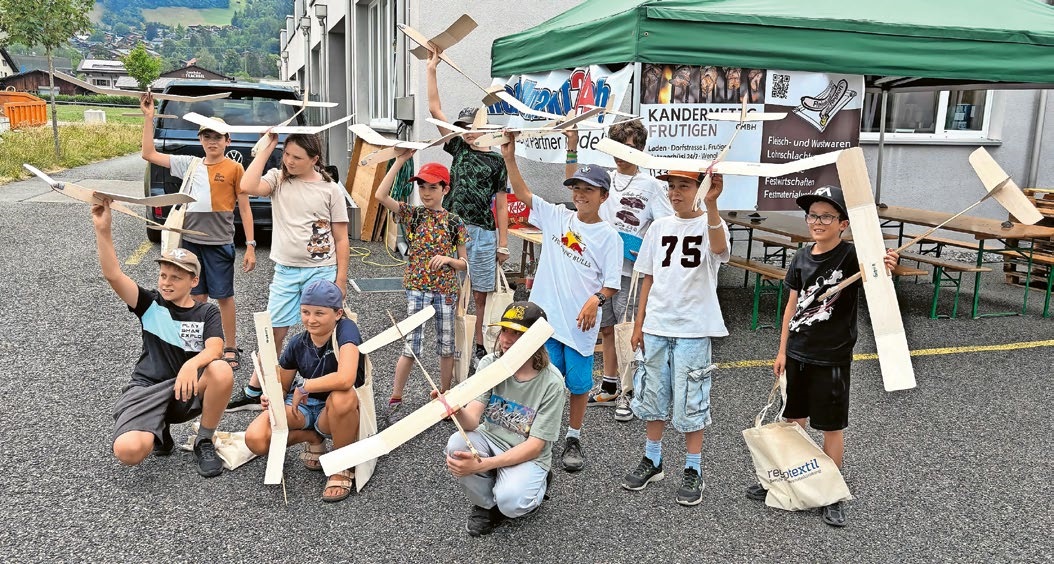
BY YOUTH, FOR YOUTH
Lorena Betschen
YOU KNOW WHAT I MEAN? 125 YEARS OF THE SWISS AERO CLUB
Emil Giezendanner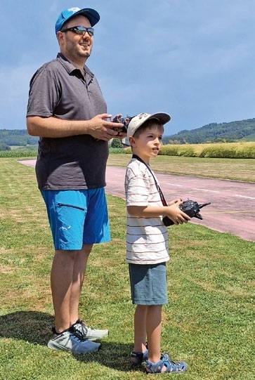
TRY-OUT DAY AT MFV WETTINGEN
Urs Keller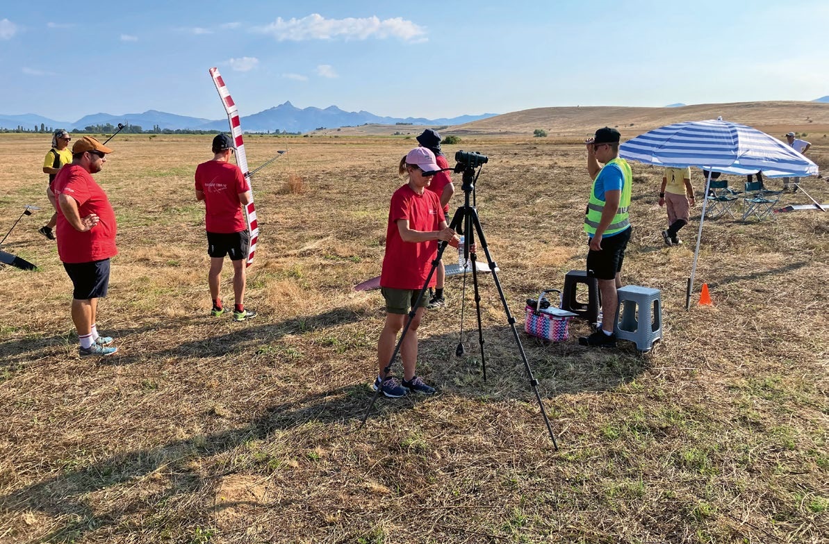
FREE FLIGHT IN THE MIDDLE OF SUMMER
Urs Muntwyler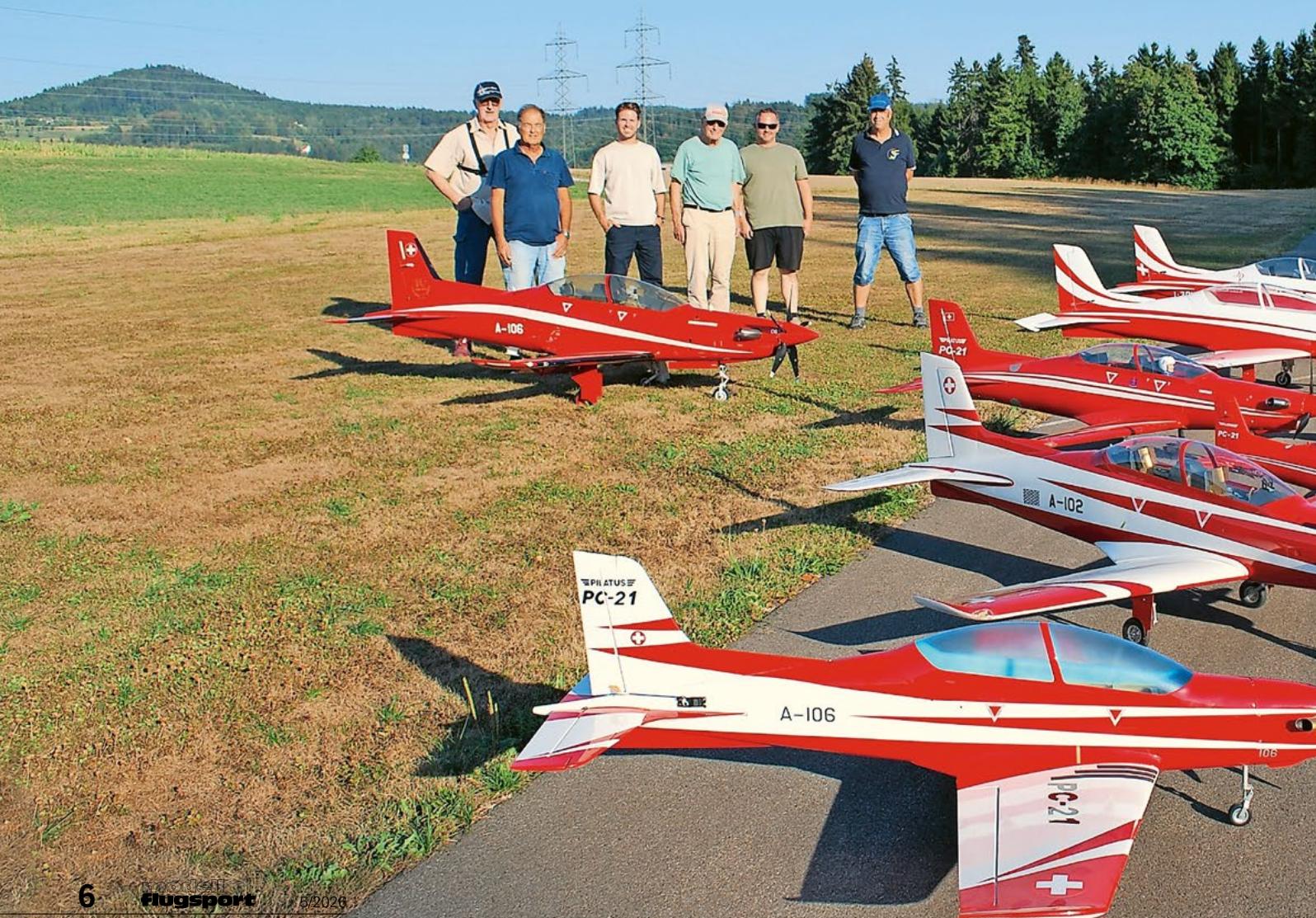
THE PC-21 STORY
Emil Giezendanner
TWIN TOWN PARTNERSHIP
Wolfgang Voeller
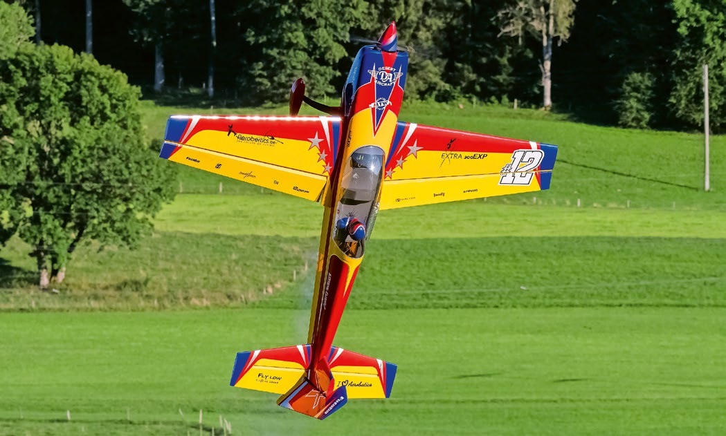
EURO CONTEST GLIDER ACRO TOUR AUSTRIA 2026
WELCOME, NEW MEMBER!
Andrea Bolliger
COUPE DES ALPES – OBSERVE AND LEARN
Rodito Nussbaumer
NEWS FROM HEBU
 Julia Bucher
FROM 0 TO 100
Markus Nussbaumer
NOS REGION – A HUB FOR ELECTRIC AVIATION
Emil Giezendanner
MEMORIES
Wolfgang Völler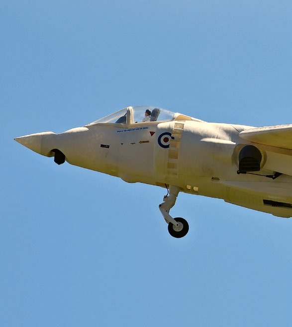
Have you almost forgotten about aircraft that take off and land vertically?
Emil Giezendanner
70 YEARS OF THE NIDWALDEN MODEL AIRPLANE CLUB
Martin Barmettler