
Modern Profiles—What's Behind Them?
Any model builder with some basic knowledge of aerodynamics and a “feel for streamlined shapes” can design a usable airfoil for their model airplane using just a pencil, compass, and curved ruler—without complicated calculations. By analyzing observations and experiments conducted on the model aircraft, a skilled model designer can refine a usable airfoil into a good one. Finding an airfoil with even better characteristics is a task that can be accomplished practically only by specialized fluid dynamics researchers using computers and sophisticated testing facilities.
Today, profiles tailored to specific applications are developed for aircraft, helicopter rotors, axial compressors, steam and gas turbines, etc.; calculating these profiles requires a design methodology based on complex computational fluid dynamics methods. The only attempt to date to adapt this modern airfoil design methodology for use in model aviation led to the well-known and widely used Eppler airfoils [1]. What insights and considerations lie behind the “computer profiles,” from which some model aviators expect miracles? This question will be addressed below, drawing in part on an American article on this topic [2].
It is not yet possible to calculate the actual flow around an airfoil, although the basic equations required for this have long been known. A solution to this problem has been sought by essentially breaking the overall problem down into two subproblems, each of which is much easier to solve on its own. In many cases, superimposing the partial solutions ultimately yields a very good approximate solution for the overall problem. All modern airfoil design methods are based on such approximations, namely the combined application of airfoil theory and boundary layer theory.
Profile theory provides either the theoretical velocity and pressure distributions around the profile, as well as the lift, for a given profile shape; or, conversely, the profile corresponding to a given velocity distribution. Boundary layer theory calculates the influence of friction and the airfoil drag caused by friction. It also specifies how the velocity must vary along the airfoil so that the airfoil drag is minimized. Some problems in airfoil theory and boundary layer theory are discussed in more detail in the following sections.
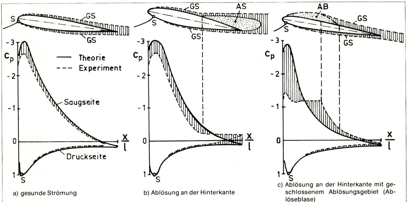
On an airfoil positioned across the flow, lift is generated because a region of reduced pressure—compared to the undisturbed flow—forms on the upper surface of the airfoil (= suction side), while on the lower surface (= pressure side), the pressure is higher than in the undisturbed flow. Figure 1 schematically shows three different flow patterns around an inclined profile.
The theory calculates the pressure distribution as if there were no friction, whereas in the experiment, measurements are taken in the actual flow. The pressure distribution curves show that the deviation between theory and experiment is small in laminar flow; see Fig. 1a. If the flow does not follow the profile surface and so-called separation or stagnant flow regions form, the theory no longer accurately reflects the actual pressure distribution; see Figs. 1b and 1c.
All computational methods used to date for airfoil design work with such idealized pressure and velocity distributions around the airfoil. For selected angles of attack, the velocity profile is specified in sections along the airfoil surface, and the airfoil that meets these specifications is calculated. What these specifications might look like will be described later. As an example of the results of profile theory, Fig. 2 shows the theoretical velocity distribution around the Eppler E 428 profile at an angle of attack $α = 8^−$. Starting from the stagnation point, where the velocity is zero and the maximum pressure head is reached ($c_p = +1$ in Fig. 1), the flow on the suction side is strongly accelerated around the leading edge of the airfoil to approximately twice the inflow velocity $v_∞$. Subsequently, the flow decelerates—first rapidly and then increasingly slowly—until about 95% of the airfoil depth. On the pressure side, the velocity increases steadily from the stagnation point up to about one-quarter of the airfoil depth. From there, it remains practically constant until the trailing edge.
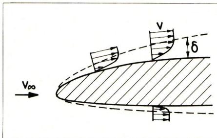
Boundary layer theory is based on the observation that, in many cases, friction manifests itself only in a thin layer along a surface—known as the boundary layer. Fig. 3 shows how, in the boundary layers formed around a slender profile, the flow is decelerated from a velocity $v$ at the edge of the boundary layer to zero right at the profile surface. Outside the boundary layer, in what is known as the outer flow, the flow behaves almost as if there were no friction.
One fundamental flow pattern of the boundary layer on a surface is the laminar boundary layer; the other is referred to as a turbulent boundary layer. Under certain circumstances, a laminar boundary layer transitions downstream into a turbulent one. This process often occurs almost instantaneously within a narrow zone and is therefore called boundary layer transition.
In the region where the flow is slowed down at the profile surface—which is always associated with a rise in pressure—the boundary layer may be forced away from the profile surface and no longer follow the contour. This phenomenon is referred to as boundary layer separation; see Fig. 1. In the case of a laminar boundary layer, even a relatively small increase in pressure can cause separation, whereas a turbulent boundary layer can withstand a larger increase in pressure.
Over time, a large number of more or less complex methods have been developed to calculate the behavior of laminar and turbulent boundary layers along the profile surface. Unfortunately, each of these methods has its advantages and disadvantages, and it is often difficult to decide which one is most appropriate in a specific case.
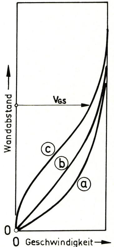
Within the laminar boundary layer, the flow is completely orderly and consists, so to speak, of layers that slide over one another. The frictional resistance of the laminar boundary layer is significantly lower than that of the turbulent boundary layer. This effect can be exploited if the boundary layer can be maintained in a laminar state over as large an area of the airfoil surface as possible. One way to achieve this is to control the development of the boundary layer through the profile shape and the associated velocity distribution in such a way that, on the one hand, the transition point is delayed as far as possible and, on the other hand, separation is prevented. The key factors here are the boundary layer thickness and the velocity at the boundary layer edge—or, more precisely, the Reynolds number—as well as the shape of the velocity profile within the boundary layer, referred to as the boundary layer profile. Typical laminar boundary layer profiles, along with information on the conditions under which they develop, are shown in Fig. 4. Boundary layer profiles without an inflection point, corresponding to examples a and b in Fig. 4, as they occur in regions of acceleration or constant velocity, prove to be particularly favorable for maintaining the laminar boundary layer. This insight led to the development of the first laminar profiles. As an example, Fig. 5 shows the velocity distributions of the unswept conventional NACA 0009 profile and the NACA 66-009 laminar profile of equal thickness. In the former, the velocity maximum occurs at about 8% and the maximum thickness at about 30% of the airfoil depth; in the latter, however, the velocity maximum occurs at about 65% and the maximum thickness at 45%.
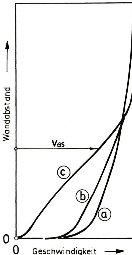
In a turbulent boundary layer, irregular fluctuations are superimposed on the average motion of the flowing medium. Although the frictional drag of the turbulent boundary layer is greater than that of the laminar boundary layer, the turbulent boundary layer can overcome a much greater pressure increase without separating from the airfoil surface. On every airfoil, there are regions near the trailing edge where pressure increases, and care must be taken to ensure that the boundary layer is already turbulent in those areas. Typical turbulent boundary layer profiles are shown in Fig. 6.
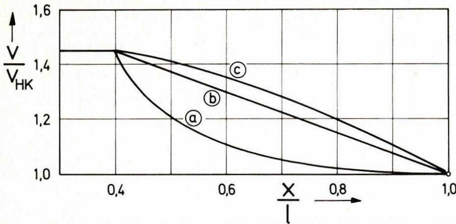
F. X. Wortmann discovered that the frictional drag of the turbulent boundary layer is particularly low when the transition is initially followed by a region with a relatively steep pressure rise and the pressure rise gradually decreases toward the trailing edge. One could also say that the turbulent boundary layer can withstand a greater deceleration shortly after the transition than later in its development. The corresponding velocity profiles are shown in Fig. 7. The exact shape of curve a is determined from calculations of the turbulent boundary layer.
The actual causes of the transition from laminar to turbulent flow have not yet been fully elucidated. Nevertheless, it has been established both theoretically and experimentally that, under certain conditions, small wave-like disturbances in the laminar boundary layer decay, and the boundary layer is stable; whereas under other conditions, these disturbances grow at certain wavelengths. In such cases, the boundary layer is said to be unstable. Further downstream, these disturbances are amplified to such an extent that the laminar state breaks down and the turbulent state sets in. The boundary between the region of decaying disturbances and the region of amplified disturbances is the indifference curve.
Figure 8 shows the corresponding indifference curve as a function of the Reynolds number $Re_\delta$ for four boundary layer profiles. The Reynolds number $Re_\delta$ differs from the Reynolds number denoted here by $Re$ , since it is defined in terms of the boundary layer thickness $\delta$ and not in terms of the chord length $l$ . Fig. 8 shows that for boundary layer profiles A, B, and C, there is a minimum Reynolds number on the indifference curve below which no disturbances are generated. This minimum Reynolds number is referred to as the stability limit of the respective laminar boundary layer. For boundary layer profile A without an inflection point, the stability limit is about ten times greater than for boundary layer profile B with an inflection point. It follows that in case B, boundary layer transition can occur at a much smaller Reynolds number than in case A. Case C corresponds to a boundary layer profile such as that which can form at the edge of a small separation bubble. Here, instability is apparently possible at an even smaller $Re_\delta$ than in cases A and B. This type of boundary layer transition has been observed specifically in the study of profiles in the field of model aircraft flight; see Fig. 9. Case D indicates the possibility of boundary layer transition at the edge of a large separation region; however, this is irrelevant for airfoil design.
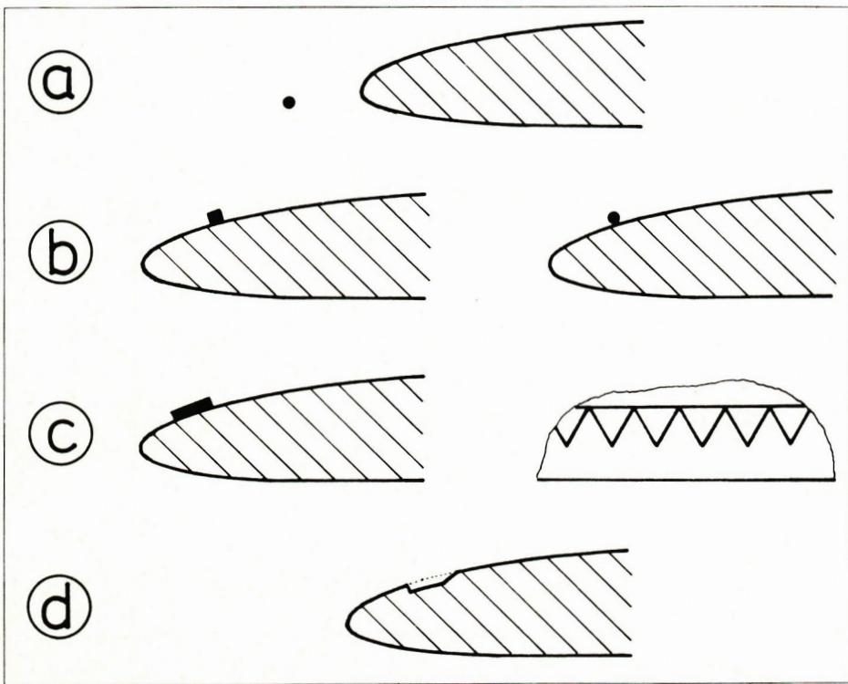
How long the laminar boundary layer can be maintained downstream after crossing the stability threshold depends on the pressure gradient, the surface texture, and the turbulence in the outer flow. When it comes to surface texture, not only the actual roughness plays a role, but also the waviness. It is well known how much attention is paid to ensuring a smooth, waveless surface in gliders. The free atmosphere is practically turbulence-free for the boundary layer at the airfoil, and the boundary layer transition is not affected. In contrast, for example, a wire stretched in front of the airfoil increases the turbulence of the outer flow so much that the boundary layer transitions shortly after crossing the stability limit; see Fig. 10a.
Further methods for influencing the transition are shown in Figs. 10b–c. They artificially induce a situation similar to that which occurs naturally with the separation bubble shown in Fig. 9. The triangular turbulator shown in Fig. 9c has proven particularly effective on free-flight models. Little is known about the effect and optimal design of a step or groove built into the airfoil surface (Fig. 9c). This groove-type turbulator, in particular, could open up interesting possibilities for radio-controlled glider models. For example, it would be conceivable to adjust the groove using a radio-controlled flap to match the airspeed and thus the Reynolds number.
The laminar boundary layer separates as soon as a boundary layer profile has formed, as shown in curve c in Fig. 4. This provides a criterion for determining the separation point. To date, it has not been possible to continue the boundary layer calculation beyond a separation point. Therefore, it is also not possible to calculate the profile drag when the flow does not adhere to the profile throughout its entire length. So far, we have only discussed the separation of the laminar boundary layer. A similar process can also be observed in the turbulent boundary layer when the pressure rise toward the trailing edge becomes too great. Strictly speaking, turbulent separation always occurs in the immediate vicinity of the trailing edge, since the trailing edge cannot be infinitely sharp. It is important that this separation region remains as small as possible over a wide range of angles of attack. The location of turbulent separation can also be predicted based on the shape of the boundary layer profile (see Fig. 6, curve c). However, the computational uncertainties are significantly greater for turbulent separation than for laminar separation.
(To be continued)


News from HEBU

TEAM MANAGER "THIS" BOSSHARD
 Rodito Nussbaumer
YOU KNOW WHAT I MEAN? 125 YEARS OF THE SWISS AERO CLUB
 Emil Giezendanner
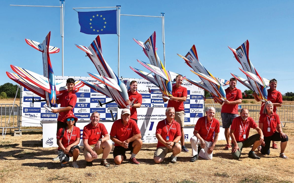
F3A EUROPEAN CHAMPIONSHIPS IN ST-MACAIRE, FRANCE
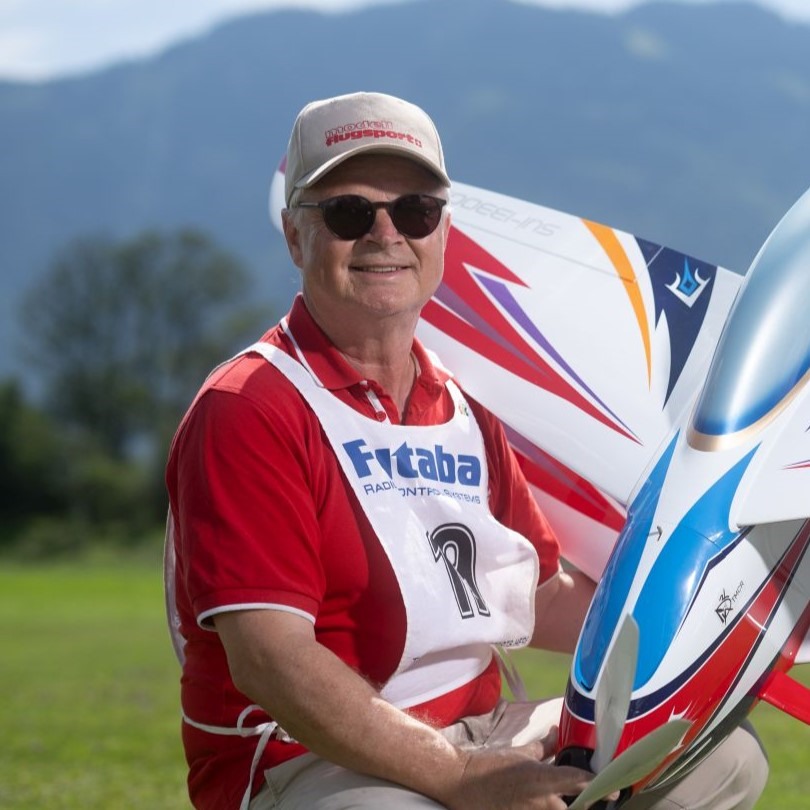 Matthias Bosshard
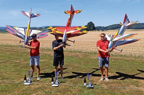
52. 2026 ALPS CUP
Emil Giezendanner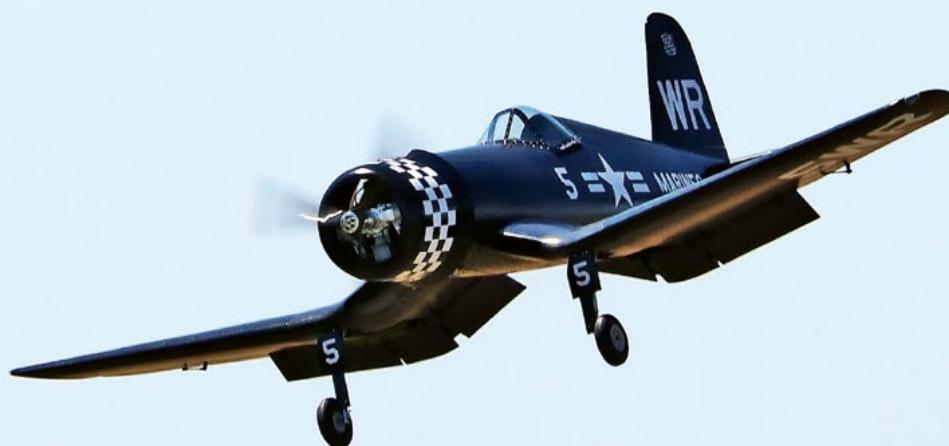
CORSAIR F4U – A WARBIRD WITH A MEMORABLE LOOK
Jürgen Rosenberger, Jürgen Prinz
SUMMER FUN 2026 AT MG USTER
Martin Wunderli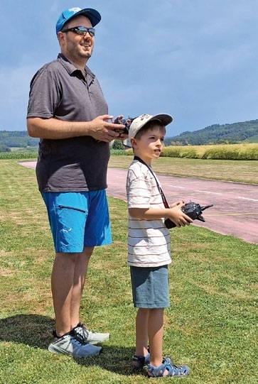
TRY-OUT DAY AT MFV WETTINGEN
Urs Keller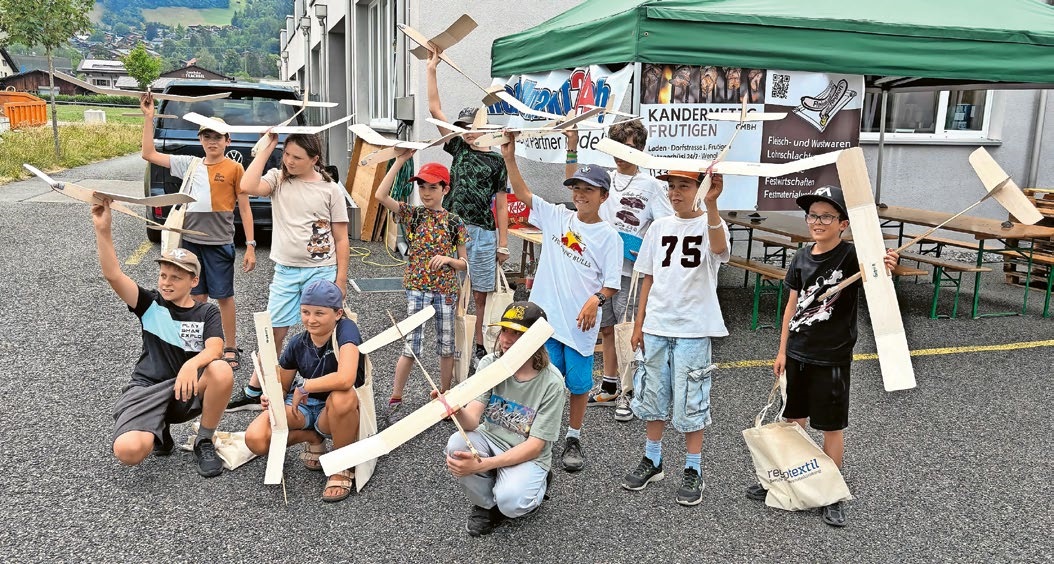
BY YOUTH, FOR YOUTH
Lorena Betschen
ATOM, THE NEW DOUBLE-DECKER FROM CPLR
Matthias Bosshard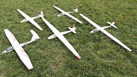
SMALL, MODEL-LIKE SAILBOATS
Res Dauwalder
What's New at Leomotion.com
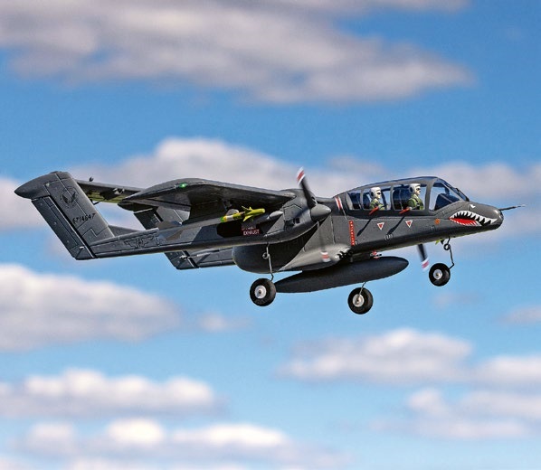
HORIZON HOBBY/LEMACO NEWS: MICRO OV-10 BRONCO 645 MM BY E-FLITE
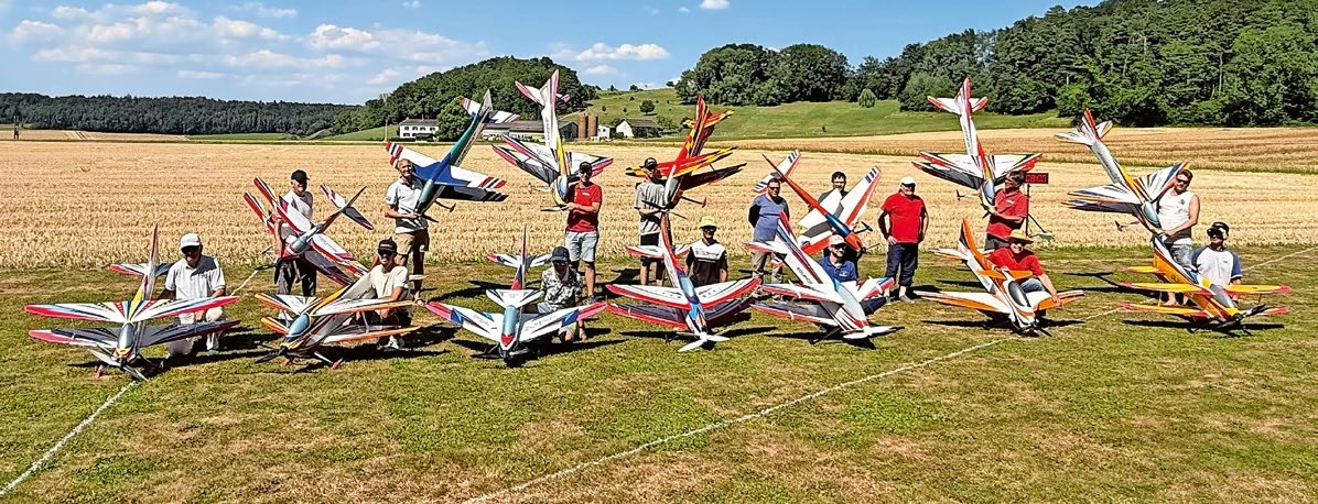
COUPE DES ALPES – OBSERVE AND LEARN
Rodito Nussbaumer
TWIN TOWN PARTNERSHIP
Wolfgang Voeller
PRIDE AND GOOD IDEAS
 Markus Nussbaumer
EURO CONTEST GLIDER ACRO TOUR AUSTRIA 2026
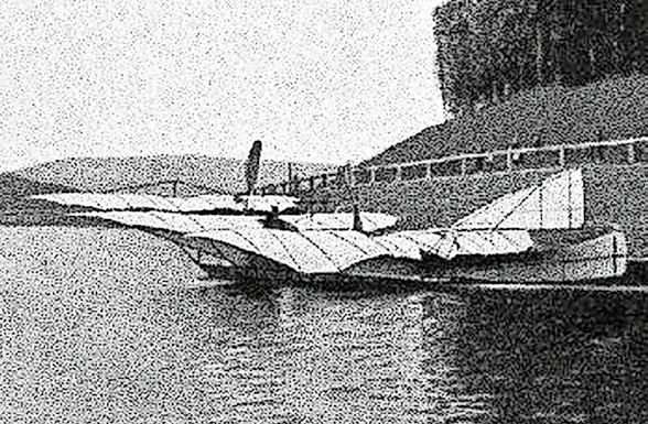
INSIGHTS INTO THE HISTORY OF SEAPLANES
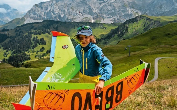
34th HAHNENMOOS ALPINE MODEL AIRPLANE CAMP
Res Dauwalder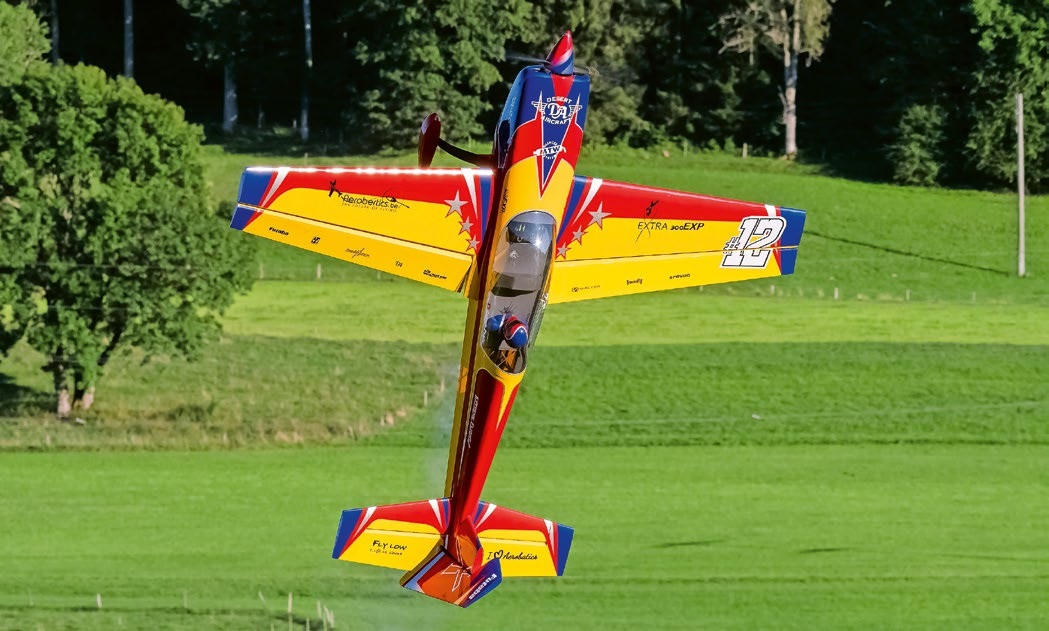
WELCOME, NEW MEMBER!
Andrea Bolliger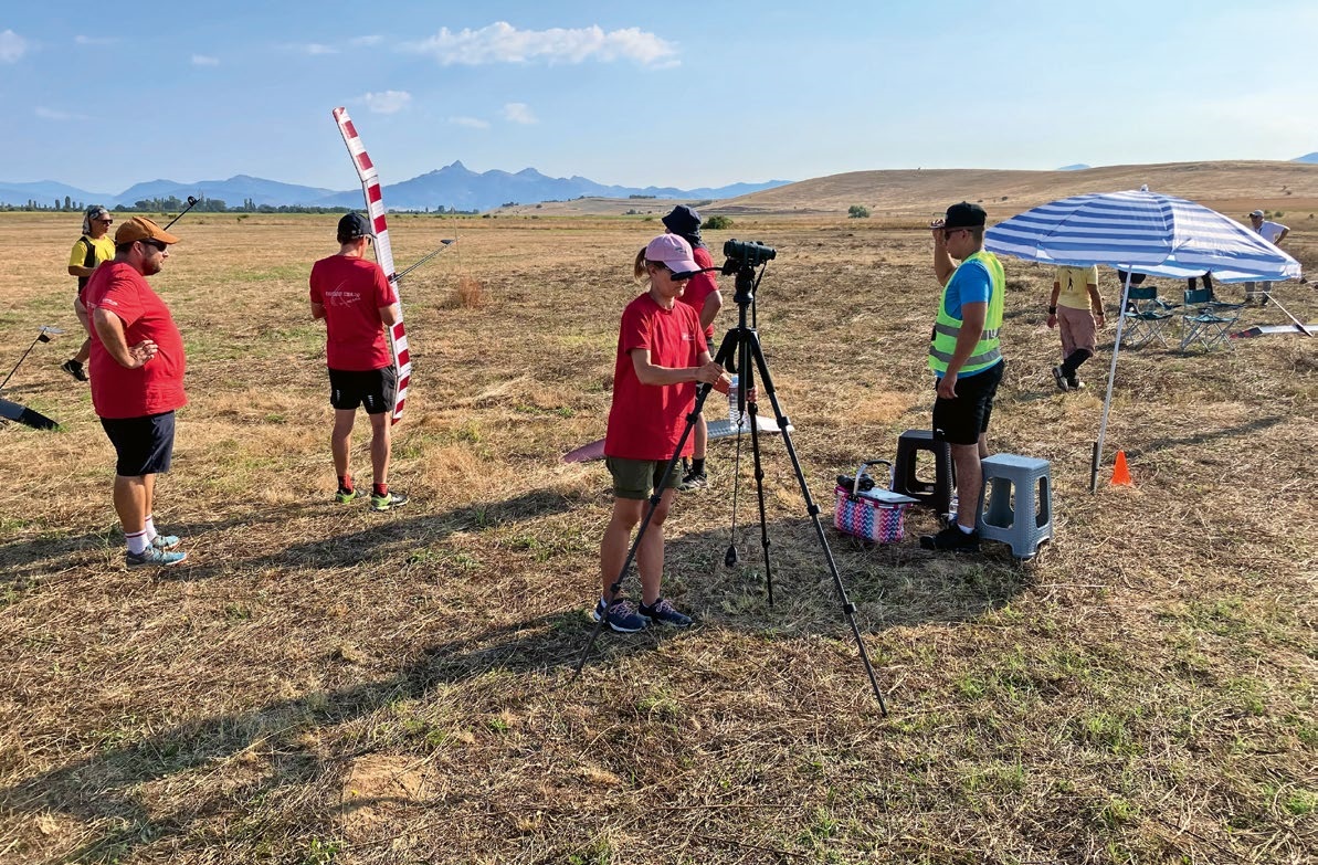
FREE FLIGHT IN THE MIDDLE OF SUMMER
Urs Muntwyler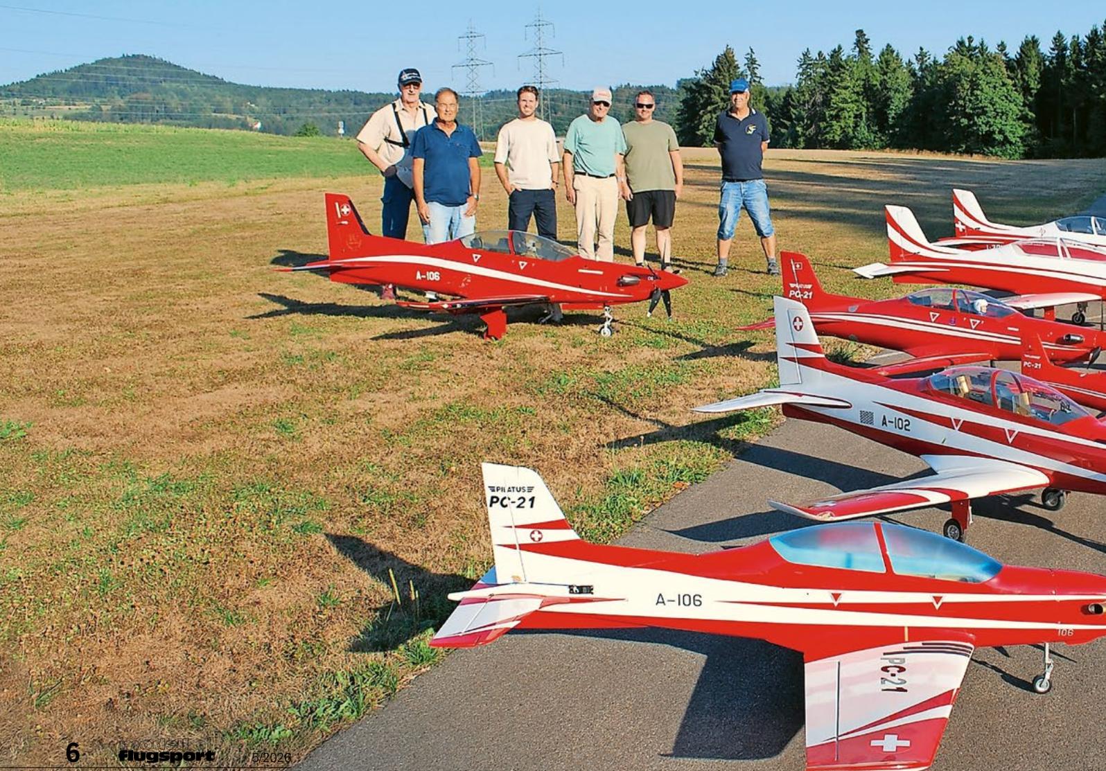
THE PC-21 STORY
Emil Giezendanner
NEWS FROM HEBU
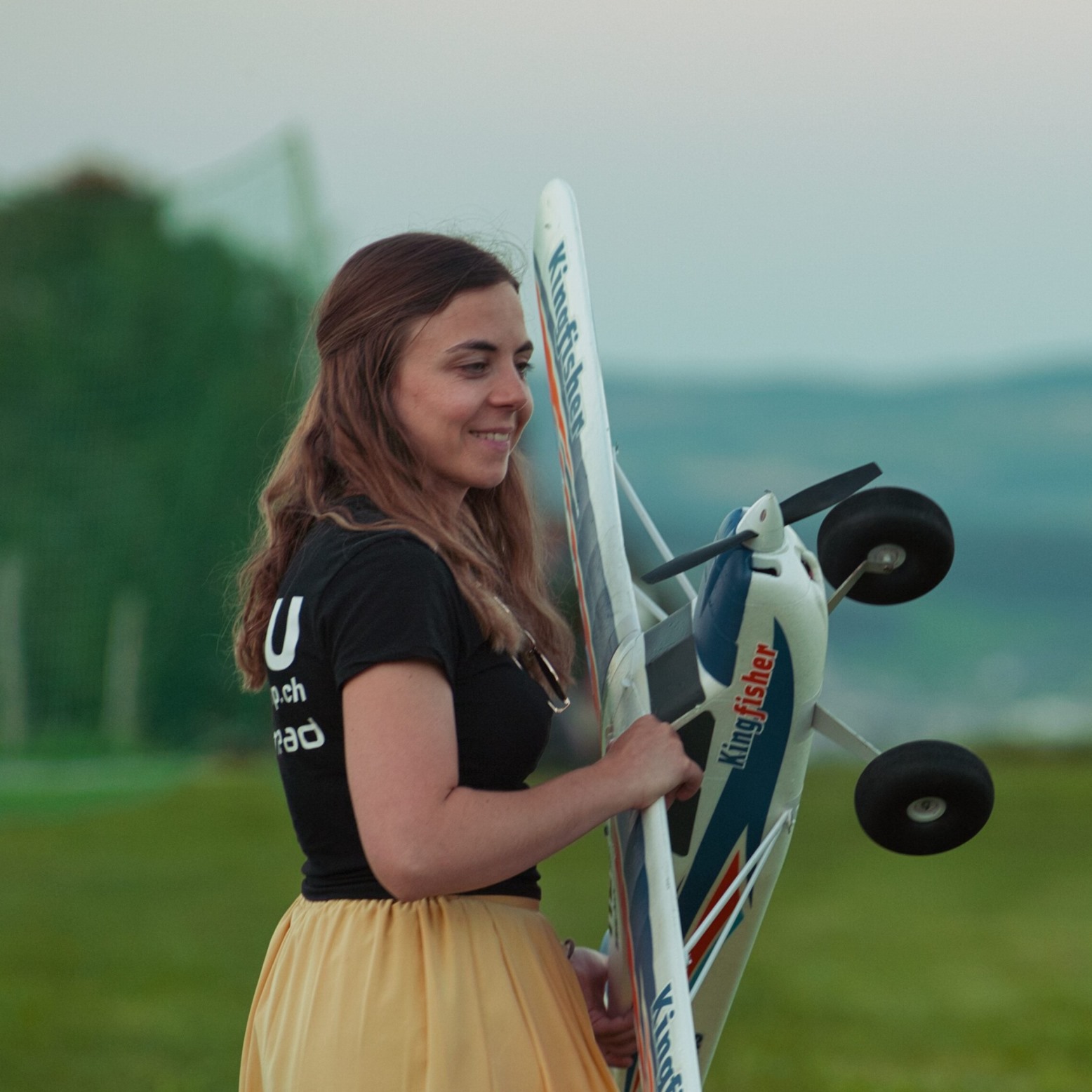 Julia Bucher
FROM 0 TO 100
Markus Nussbaumer
MEMORIES
Wolfgang Völler
NOS REGION – A HUB FOR ELECTRIC AVIATION
Emil Giezendanner
Have you almost forgotten about aircraft that take off and land vertically?
Emil Giezendanner
DO YOU KNOW WHAT I MEAN IN THE LAND OF SMILES?
Emil Giezendanner